Task 1
Spreadsheets are frequently used to record information and perform
calculations on the results of investigations and experiments. In
mathematics, spreadsheets are particularly useful when a number of
repetitive calculations need to be performed. The main features of the
Microsoft® Excel spreadsheet are described below. Open a new Excel
spreadsheet to help you identify the features described.
Rows, columns and cells
- Horizontal rows are labelled 1, 2, 3, 4, … and vertical columns are
labelled A, B, C, D, …
- The intersection of a row and a column is called a cell.
- The cell at the intersection of column A and row 1 is referred to as A1.
- The highlighted rectangle on the screen is called the cell pointer
and the cell containing the cell pointer is called the active cell.
- Note that Excel contains 256 columns labelled A, B, C, …, AA, AB, …,
AZ, …, BA, BB, BC, …, BZ, CA, CB, CC, …, CZ, …. and it contains 65
536 rows labelled from 1 to 65 536.
Standard toolbar
The Standard toolbar provides easy access to frequently used functions
such as save, cut, copy, paste, etc.

Formatting toolbar
The Formatting toolbar provides easy access to commands such as bold,
italics, font, alignment of text, etc.

Creating a simple worksheet
Two of the data types that can be entered into the individual cells of
the worksheet are:
- Text (labels) - used to make a worksheet more readable by identifying
rows and columns.
- Numbers (values) - the numeric characters 0, 1, 2, 3, 4, 5, 6, 7, 8
and 9 are used to write numbers in the cells. The numbers can also begin
with a + or – symbol.
Task 2: Entering data into a worksheet
The points won by David and Peter in table-tennis match are shown in the
table below.
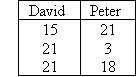
On your spreadsheet, enter this data as follows:
- To key in David, move the cell pointer to B1
and type David. Then press Enter.
- To key in Peter, move the cell pointer to C1
and type Peter. Then press Enter.
- To key in 15, move the cell pointer to B2
and type 15. Then press Enter.
- To key in 21, move the cell pointer to B3
and type 21. Then press Enter.
Similarly, we can enter the remaining data.
Editing techniques
- To erase a mistake made while keying in data, use the Backspace
key.
- To replace data already entered with other data, move the cell pointer
to the cell and type the new data. Then press Enter.
The new data will be displayed in the cell.
Erasing the contents of a cell
To erase the contents of a cell, move the cell pointer to the cell
concerned and press the Delete key. Note that
if data is deleted accidentally, the last item deleted can be recovered by
pressing Ctrl + Z
or by clicking the Undo button.
Formulas
Numerical data is manipulated by using a formula.
For example, =B2+B3+B4 is a formula that
will add the contents of cells B2, B3,
and B4.
Note that if the first keystroke is not the equal sign (=), Excel will
assume that you have entered a label and will not calculate a formula.
A formula is an instruction given to Excel to make it perform
calculations. In the example above, a formula is used to add the contents of
the cells. Now, we will create formulas for performing subtraction,
multiplication and division of the contents of two or more cells.
The formula bar contains the formula or cell contents in a cell and can
be used for editing a cell's formula. To find the formula bar, repeatedly
select Formula Bar from the View
menu in Excel until you can identify it.
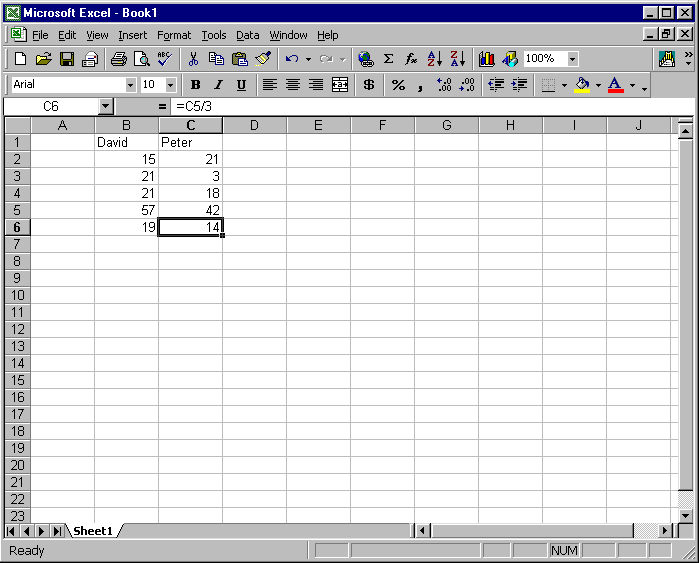
Adding the contents of the cells
To find the sum of the points scored by David, move the cell pointer to B5
and key in the formula =B2+B3+B4.
Then press Enter.
The sum 57 is displayed in cell B5.
Likewise, to find the sum of the points scored by Peter, move the cell
pointer to C5 and key in the formula =C2+C3+C4.
Then press Enter.
The sum 42 is displayed in the cell C5.
Finding the average of the contents of the cells
In the example above, to find the average number of points scored per
match by David, move the cell pointer to B6 and
key in the formula =B5/3. Then press Enter.
The average score, 19, is displayed in cell B6.
Likewise, to find the average number of points scored per match by Peter,
move the cell pointer to C6 and key in the
formula =C5/3. Then press Enter.
The average score, 14, is displayed in cell C6.
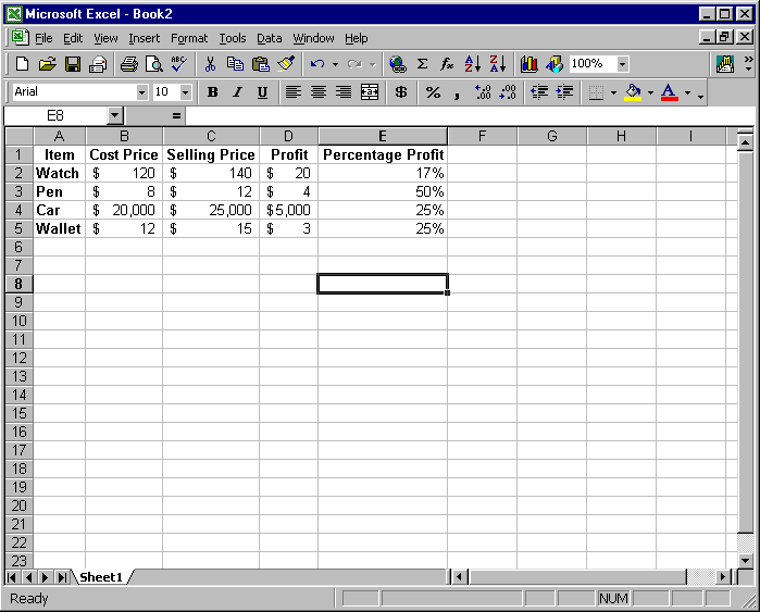
Subtracting the contents of the cells
The cost price and selling price of some items are recorded in the
following table.
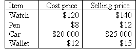
Open a new spreadsheet and record this information in cells A1
to C5.
To find the profit made by buying and selling a watch, move the cell
pointer to D2 and key in the formula =C2-B2.
Then press Enter.
The difference of $20 is displayed in cell D2.
Likewise, to find the profit made by buying and selling a pen, move the
cell pointer to D3 and key in the formula =C3-B3.
Then press Enter.
The difference of $4 is displayed in cell D3.
Similarly, we can find the profit made on the other items.
Multiplying and/or dividing the contents of the cells
To find the percentage profit made by buying and selling a watch, move
the cell pointer to E2, key in the formula =D2/B2,
press Enter and click the %
symbol on the Formatting toolbar.
The percentage profit of 17% is displayed in cell E2.
Likewise, to find the percentage profit made by buying and selling a pen,
move the cell pointer to E3, key in the
formula =D3/B3, press Enter
and click the % symbol on the Formatting
toolbar.
The percentage profit of 50% is displayed in cell E3.
Similarly, we can find the percentage profit made on the other items.
Improving the appearance of a worksheet
The appearance of a worksheet can be improved by formatting cells.
To format a cell (or a group of cells), we need to select it first as
described below.
Selecting a cell
To select a cell, position the cell pointer over it and click the left
mouse button. The selected cell will have a border around it.
Selecting a group of cells
A group of cells is selected either by the dragging or shift-select
method.
- Dragging - Place the cell pointer in the first cell and hold down the
left mouse button (LMB). Then drag the cell pointer through to the end
of the group of cells and release the mouse button. Note that the LMB is
held down while dragging.
- Shift-select - To select a group of cells, point and click on the
first cell. Then hold down the Shift key
and point and click in the last cell.
Selecting a group of non-contiguous cells
To select a group of non-contiguous (i.e. unconnected) cells, point the
mouse cursor and click on the first cell (or group of cells). Then hold down
the Ctrl key and point and click to select
further individual cells.
Note that you can select further individual cells or a range of cells by
dragging while holding down the Ctrl key.
Task 3
Use the dragging method to select the cells from
(a) A1 through to A10
(b) C5 through to C10
(c) B4 through to B15
(d) E3 through to E12
Task 4
Use the shift-click method to select the cells from
(a) A1 through to A15
(b) C2 through to C14
(c) B5 through to B112
(d) E6 through to E10
Changing the column width
To reset the column width, drag one of the lines that separates the
column headings (to the left or right) or double click one of these lines to
set auto column width.
Changing the row height
To reset the row height, drag one of the lines that separates the row
headings (either up or down) or double click one of these lines to set auto
row width.
Task 5
- Reset the width of columns A, B, C and D.
- Reset the heights of rows 1, 2, 3 and 4.
Aligning text
The Formatting toolbar provides the option to left, centre, and right
align text and also merge and centre cells. To align text, highlight the
cells you want to align. Then select the desired alignment button from the
toolbar.
Task 6
Use a spreadsheet to find the value of:
(a) 625 + 25
(b) 625 – 25
(c) 625 ´ 25
(d) 625 ¸ 25
(e) The average of (a) to (d).
(f) Save the file and print the worksheet.
Solution:
Open a new spreadsheet and enter 625 in A3
and 25 in B3.
Position the pointer in D3. Then type the
labels
A3 + B3 = in D3,
A3 - B3 = in D4, A3
* B3 = in D5, A3 /
B3 = in D6 and average
= in D7. Align the contents of the cells
D3 to D7 to the
right.
(a) Enter the formula in E3 to compute
the sum of 625 and 25.
(b) Enter the formula in E4 to compute
the difference of 625 and 25.
(c) Enter the formula in E5 to compute
the product of 625 and 25.
(d) Enter the formula in E6 to compute
the 625 ¸ 25.
(e) Enter the formula in E7 to compute
the average of the given numbers. Remember BODMAS for your formula for
average.
Task 7
Change the value of A3 to 100
in the spreadsheet created for Task 6. Observe the effect on the values in
the cells E3 to E7.
Choose the Save As option from the File
menu to save the file under a different name and print the worksheet.
Printing formulas
To check the formulas used in the worksheet, select Options
from the Tools menu. Then select Formulas
from the View tab and select OK.
The formulas of the worksheet will be displayed. Alter the column widths
in order to format the worksheet to fit the screen. Save the file and print
the worksheet. To display the values of the worksheet again, select Options
from the Tools menu. Choose the View
tab and clear the Formulas check box.
Task 8: Fractions
We can add, subtract, multiply, and/or divide fractions by using a
spreadsheet.
Use a spreadsheet to evaluate the following fractions:


Solution:
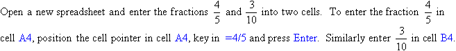
You can format these cells as fractions by selecting Fraction
format by choosing the Cells option of the Format
menu and selecting the Number tab and finally Fraction.
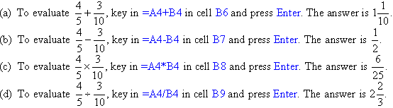
Print and save the file.
Task 9: Order of calculations
If x = 4, y = 6 and z = 2, use an Excel spreadsheet
to calculate the following:
(a) xy
(b) x ¸ z
(c) xy + z
(d) xz – y
(e) y ´ z ¸
x
(f) x – y ¸ z
(g) (x + y)z
(h) (y – x ¸ z
) ¸ x
Solution:
Remember BODMAS when entering your Excel formula.
Enter 4 in cell B3,
6 in cell B4 and 2
in cell B5.
(a) To calculate xy, enter the formula =B3*B4
in cell B7.
(b) To calculate x ¸ z,
enter the formula =B3/B5 in cell B8.
(c) To calculate xy + z, enter the formula =B3*B4+B5
in cell B9.
(d) To calculate xz – y, enter the formula =B3*B5-B4
in cell B10.
(e) To calculate y ´ z ¸
x, enter formula =B4*B5/B3 in cell B11.
(f) To calculate x – y ¸ z,
enter formula =B3-B4/B5 in cell B12.
(g) To calculate (x + y)z , enter formula =(B3+B4)*B5
in cell B13.
(h) To calculate (y – x ¸ z
) ¸ x, enter formula =(B4-B3/B5)/B3
in cell B14.
|